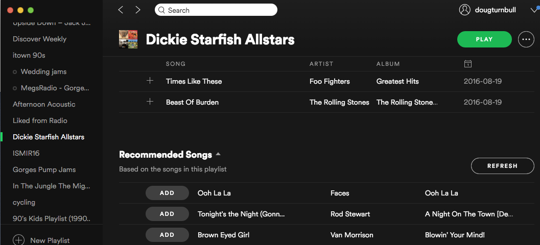
Having returned from Singapore with a few months left in my sabbatical and without having MegsRadio to focus on, I found myself with a few months to work on a couple of new projects. One of these projects was to compete in the 2018 ACM RecSys Spotify Playlist Challenge which recently ended on June 30th.
Background:
ACM RecSys is the top academic conference on recommender systems research. Each year they host a data mining competition to spur innovation and drive interest in the field. This year they teamed up with Spotify to create a competition that focused on playlist algorithms. The basic setup is that they give you 1 million user-generated playlists called the Million Playlist Dataset (MPD).

They provide another challenge dataset with 10,000 user-generated playlists but where some faction of the songs is removed. The goal is to predict the missing songs. More specifically, for each of the challenge playlists, a playlist algorithm makes 500 song predictions from the set of 2.3 million unique songs in MPD.
Playlist Embedding:
The core of my approach was to use Latent Semantic Analysis (LSA) to embed playlists into a (128) dimensional space. We start by representing the MPD as a playlist-by-song matrix. (The dimensions of this matrix would be 1M playlists by 2.3M tracks so it is important to represent it as a sparse matrix.) We then learning an embedding using singular value decomposition (SVD) that re-represents each playlist in a much smaller (but dense) vector of numbers. These, say 128, are an embedding that is a much more compact representation of a playlist. The cool thing is we can also back-project one of the 128-dimensional embedded vectors back into the original 2.3M dimensional space such that the error between this new vector and the original vectors has as little (squared) error as possible.
We can then take a playlist from the challenge data set, projects it into the low-dimensional space and then back-project into the 2.3M dimensional space. Finally, we rank all of these 2.3M values (not including the values associated with the songs that are already know to be present in the playlist) and keep the top 500. These 500 dimensions then become our top candidates for the 500 missing tracks.
Playlist Titles:
Another important aspect of the playlist datasets is that most playlists come with some sort of text-based title (e.g., “Sunday Morning”, “High Energy Workout Mix”, “My Jams”, “Blues”, etc.) About 10% of the playlists in the challenge dataset came with a title and no tracks and another 10% came with the title and one track so it was important to use the textual information to make song predictions. The good news is that I teach a course on information retrieval and this is a pretty standard setup for how one might implement a simple text-based search engine.
However, unlike web pages, playlist titles short so we are not dealing with much textual content. We also want to rank songs (as opposed to similar playlists) so we had to be a little clever. To solve these two problems, I represented each song as a concatenation of all of the titles for all of the playlist that the song appears on. This means that each song is represented as a long document of playlist titles. we then apply a number of standard information retrieval tricks: stop-word removal, term-frequency-inverse-document-frequency scaling, document length normalization, etc.
Finally, for each challenge playlist, we use the title as a “query” and use it to rank all of the 2.3 million tracks. More specifically, we compute the cosine distance between the challenge playlist title and each of the “song document” which produces relevance scores between 0-1.
Additional Information:
As with most recommender systems, there is usually a large popularity bias. That is, a small number of popular songs show up on a large number of playlists while most songs show up only on one or two playlists. For example, the most common song “Humble.” by Kendrick Lamar shows up on 4.7% of the playlists whereas 64% of the songs show up on less than 0.0001% of the playlists. To model this popularity bias, we compute the prior probability of each song showing up a playlist.
We also observe that if there is one song from an artist on a playlist there is likely to be other songs by that artist. This is also the case for albums. To model this, we keep track of the top 5 songs by each artist and the top 5 songs on each album. Then for all of the artist and albums that appear on challenge playlist, we can create a larger set of related songs by taking the union of all of the top 5 artist and album sets.
Combining Information with Bayesian Optimization:
For each training playlist, we have four vectors over the 2.3 million dimensional space:
- Playlist Relevance: vector of values computed by embedding and unembedding using LSA
- Title Text Relevance: vector of cosine distances between challenge playlist title and all song documents
- Popularity Bias: global prior probabilities of each song appearing on any given playlist
- Related Songs: a binary vector for top songs for the artists and albums that appear on the challenge playlist
We then combine these vectors as a linear combination where each vector is first multiplied by a weight and then they are added together. Rather than set these values by hand, I use Bayesian Optimization to learn these weights. Here is a summary from Fernando M. F. Nogueira, the authors of the software package:
Bayesian optimization works by constructing a posterior distribution of functions (Gaussian process) that best describes the function you want to optimize. As the number of observations grows, the posterior distribution improves, and the algorithm becomes more certain of which regions in parameter space are worth exploring and which are not.
Once we have combined the vectors, we zero out all of the dimensions that are associated with songs that appear in the challenge playlist. We then rank order all of the dimension, keep the top 500 songs, and write it to our output prediction file. This file is upload to the ACM RecSys Spotify Challenge website for evaluation.
Evaluation:
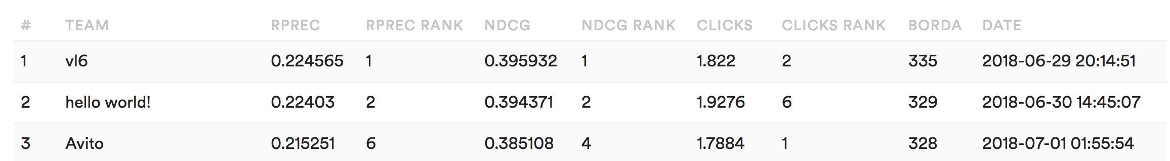
The competition organizers picked three evaluation metrics (R-Precision, NCDG, Clicks.) Without going into detail, they all measure how good the playlist algorithm is at predicting and ranking the missing songs. These three scores are then used to rank the 113 entries and the rankings are combined using the Borda score to arrive at a final ranking of playlist algorithms. Here are the top 5 teams and my “JimiLab” performance (48th place overall):

Reflection:
At the outset, I had hoped to do better (top 10) but sadly there is a significant gap between my performance and the top teams. The good news is that the top teams are required to publish a description of their algorithms along with links to their code repositories in order to be eligible for awards (recognition and $$$.) I can’t wait to see what they all cooked up. I suspect there will be a lot of deep learning (the good) as well as a lot of customized hacking for specific challenge playlist (the bad).
Having spent a good deal of time with the Million Playlist Dataset, trying out alternative predictive algorithms, developing internal evaluation code, and submitting daily result predictions, I gained a lot of perspective on playlist evaluation in general. In particular, one of the mistakes we made with MegsRadio was diving right into app development without truly exploring and evaluating our playlist algorithm. This is something I plan to rectify in future iterations of our local music recommendation systems.